Example: Fitting a surface to a boundary curve and developing (flattening) the surface into a 2D pattern.

1. Start the Pilot3D program.

2. Pick the ‘x’ boxes on three of the four views to get ready to load an existing file. I personally don’t like the 4 views on the screen at the same time. You can maximize one window at a time, but I like to use just one window. (The program can be changed to start up with just one window by changing to the Set4View=n setting in the INI file.) With one window left, maximize it to fill the entire screen.

3. Pick File-Data File Input-DXF Input. We will read some geometry from a standard DXF geometry file. This file will contain the boundary information of a surface where the boundary is defined as a series of connected points – a polyline. When you select this command, a dialog box with DXF input options appears.

4. If you are not exactly sure what is in the DXF file, don’t change any of the DXF input options and just pick the OK button. The program will read the DXF file and tell you how many entities of each type are found. The program also creates a text (TXT) file that gives you full details.

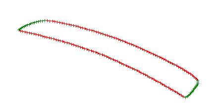
5. Display the boundary curve in the Top View. It should look like this:

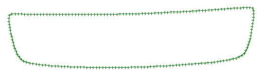
I need to provide a little background discussion. You can’t develop or layout a curve from 3D to 2D. There are an infinite number of possibilities. You first have to define a surface inside of the boundary curve. The best bet would be to have some cross-section curves between the two long sides that describe the inside shape. Without this information, the best guess is to assume that the shape of the surface in one of the two directions is straight or flat. For this “wireframe” model, the assumption is that the surface is straight going between (perpendicular to) the two long edge curves.

Now that I have made this observation, I need to know how to fit or create a surface in this area. There are many ways to create surfaces in Pilot3D, but the most convenient way to do this is to fit, skin, or loft a surface (membrane) across or through two or more curves. I will use the Create 3D-Skin/Loft command to pick two or more curves to fit with a surface. These curves that are fit will form a series of cross-sections of the model. For this boundary curve, the simplest approach is to fit a surface between the two long edges of the boundary or fit a surface between the two short edges of the boundary. If only two opposing edge curves are used, then one would want to use the two long edges because the surface between them is flat – at least that is our guess/approximation.

Now, let’s go back to the details. The curve that is drawn turns out to be one entity – a polyline. (In a CAD program, an entity is one of the lowest types of geometry that can be created and edited as one unit.) I know that it is one entity by using the Highlight Entity command.

6. Select the View-Highlight Entity command and pick anywhere on the boundary curve. Since the whole curve changes color (temporarily), then that indicates that it is a single entity or unit of geometry. When you use the View-Redraw View, the entity will be redrawn with its original color. We now want to find the start/end points on the polyline entity so that we can break the single boundary polyline into four separate side polylines.

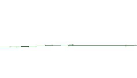
7. Looking at the full view of the boundary curve, it’s not clear where the start/stop point is located. Select the Zoom command (the magnifying glass icon on the toolbar) and pick/drag a rectangular box close to the curve at some point. Then, use the scroll bars to traverse the single boundary curve to find the start/stop point. That is the place where there is a gap and the two ends don’t meet up exactly. (Note: when you are digitizing the object, put in one extra point that is not on the boundary so that it is easy to see where you stopped digitizing. I found the gap in the middle of the upper boundary edge, as shown below.

What you want to do is to break the single polyline boundary entity at the four corners and then join the top two boundary edge pieces at this start/stop point. You want a separate polyline entity for each side of the boundary.

8. Select the Curve-Break curve command and pick one of the points in each of the four corners. It is not overly critical which point you pick because you will need to fix up the corners later.

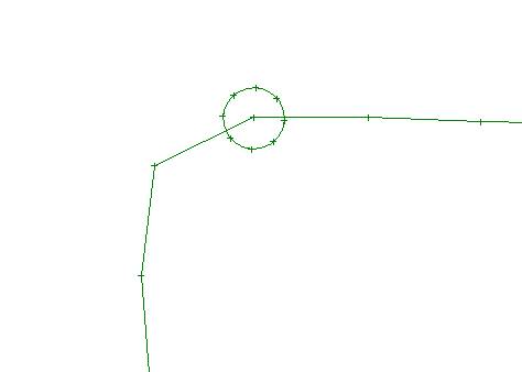
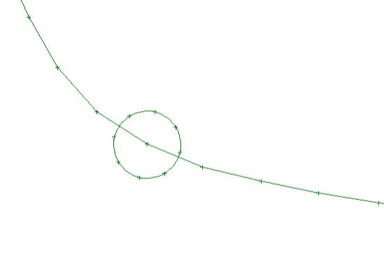
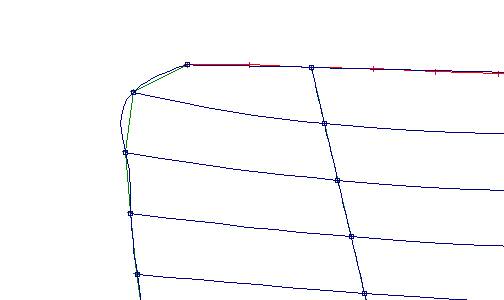
This is a snapshot of the upper left corner in the Top View. I drew (for show only) a circle at the point I used to break the long boundary polyline. You do not have to put a circle here to use this command. (If you are curious, I used the Create 2D-Circle-Center+Radius command.)

Note that when you select almost any command in this program, it stays on or current (see the box in the lower right of the screen). This means that when you pick each of the four corners to break the polyline entity, you don’t have to select the command each time. One of the exceptions to this rule is the Zoom command (the magnifying glass on the toolbar), which only works one time and the previous command stays current. This allows you to select the Curve-Break command and zoom in on each corner without having to reselect the Curve-Break command.

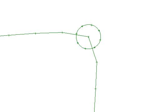
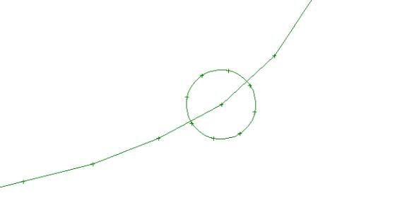
This is the point I “broke” at the upper right corner.

This is the lower left corner I broke in the Top View.

This is the lower right corner point I broke in the Top View.

Now, all four corners have been broken, but we have five entities because the top boundary curve is still broken in two pieces. You have to join the two pieces together. This is done in two steps. First, you have to merge or match up the end of one dangling polyline with the end of the other polyline. Second, you have to use the Curve-Join command to actually convert the two separate entities into one.

9. Zoom in on the point where the original start/stop point is located.

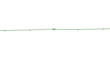
This shows the start/stop point on the top boundary edge that has to be joined together.

10. Select the Edit-Match Point-3D Match command. Pick (left mouse button) the dangling point (start or stop) of one curve and then pick the other dangling end. The program will move the first point to be exactly equal to the second point.

11. Select the Curve-Join command and pick the now matched up points. The program will then convert the matched up, but two polyline entities into one, single polyline entity.

OK, Now you are finished with the initial set-up phase. To make it clearer that you are working with four separate polyline entities on the four edges, you should change the color of two opposite sides of the boundary. (or, you can give each edge a different color.)

12. To change the color of any entity, position the cursor on the entity and pick the right mouse button. Be careful not to pick too close to an edit (+) point because the program will think that you want to know the position of that point. For a curve, you want to pick a point in-between two edit points. If the program pops up a dialog box giving you the [X,Y,Z] coordinates of the point, then you picked too close to a point. You may have to zoom in and then pick the curve. If done correctly, the program will pop up an attribute box for the entity where you will see a button that will change the color of the entity. 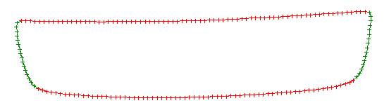Pick the color button and change the color to red. 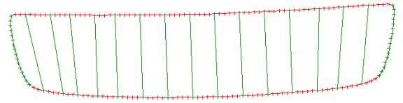Do this for the upper and lower boundary edge curves. When you are done, you will see something like this:

13. To get a better idea of the shape, you can display it in the 3D view (see the button on the toolbar) and use the other buttons to rotate the model about the Z-axis or rotate the model up or down. This is one particular view.

3D View of the four boundary edge polylines.

We are going to use the Create 3D-Skin/Loft Surface command to fit a surface to these curves. This can be done in either direction, using the two opposing long edges or the two opposing short edges. Fitting a surface directly (straight) between the two short (green) edge curves doesn’t make sense because it will ignore the shape of the two long (red) edge curves. The better bet is to fit a surface between the two red long edge curves (Oops, sometimes I use curve when I really mean polyline.) This will work, but it won’t follow the shape of the two short (green) edge curves. Remember that the skin/loft command will fit a surface straight between the two red edge curves and will not know anything about the two green edge curves. This isn’t too bad because you can always fix-up (edit) the surface after it has been created to match the shape of the green end curves.

However, we can do better without too much effort. What if we create some straight lines that cross between the two long, red edge curves. Then we can skin a surface from one short, green, edge curve, through the intermediate cross lines or curves, all the way to the opposite short, green edge curve. This would give us a good fit of all edges of the digitize boundary. To do this, we are going to add polylines and snap them to opposing points along the two long, red boundary curves.

14. Select the Curve-Add Polyline command. (Keep in mind that for Pilot3D, lines, polylines, and curves are all variations of the same type of entity – a curve.) The normal way that this command works is by using the left mouse button to pick positions on the screen where you want to add the next point of the polyline. When you are done, you pick the right mouse button. For our case, however, we want to “snap” each end point of a line (a polyline with just two points) to two opposing points along the long, red boundary edge curves. This is done using the ‘p’ key on the keyboard rather than the left mouse button.

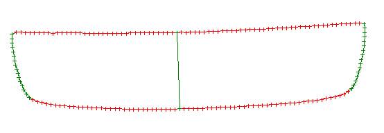
OK, the first cross-surface line we will insert will be in the middle of the two long, red edges. (We are going to add in a bunch of these cross-lines, so we will start in the middle and then keep subdividing the distances in half.) Position the cursor at (about) the middle point of the top curve and press the ’p’ key on the keyboard. Next, position the cursor in about the same location of the opposite long, red boundary curve and press the ‘p’ key. To terminate the input of the polyline, pick the right mouse button. You have just defined a line in the middle between the two long edges. This should look like this below.

If you want, you can display and rotate this shape in the 3D view just to make sure that the line was really snapped to the two points.

As I said before, this is a quick operation, so we will add in a bunch more of the cross-surface lines.

15. Add in two more snapped lines half way to the two ends. Remember that the Curve-Add Polyline is still current, all you have to do is position the cursor to a new point and press the ‘p’ key. When you have added the two new lines, the model should look like this.

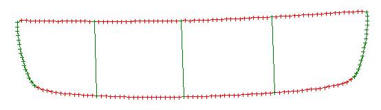
16. Add four more cross-surface lines by splitting the difference between the existing lines. You should see something like the following.

Notice that the lines added near the ends of the surface were added in with a slight angle. The reason for doing this is that I want these lines to reflect the angled shape of the two short, green end curves. We could stop now, but the process is very quick and more cross-surface lines will help you get the surface to fit the boundary edge better.

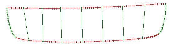
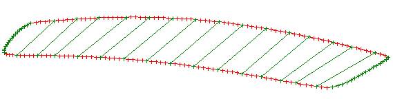
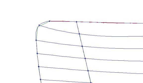
17. Add in eight more cross-surface lines by splitting the difference between the existing lines. You will end up with something like this.

Notice again that the lines near the ends of the surface reflect the change in angle of the short, green edge curves. Fitting surfaces to curves always works better if your skin/loft lines are evenly spaced.

18. Display the wireframe model in the 3D view and you should see something like this:

Remember that we don’t have a surface yet. All we have are 3D lines and polylines in space (wireframe). We will create the surface by using the short, green end edge curves and the in-between straight, green, crossing lines.

Now, if we use the end curves and the short, cross-surface, lines we have just entered, we will create a surface that matches the shape of the end curves AND will match the shapes of the two long, red boundary curves.

19. Select the Create 3D-Skin/Loft Surf command. The program will prompt you (see the status line at the bottom of the screen) to pick the curves you wish to skin – in order. Start at one end (short, green edge curve) and use the left mouse button to pick (select) the polyline. Pick the polyline near one end or the other. Next, pick the closest cross-surface line (one that you entered) NEAR THE SAME END as the first polyline you picked.

[Note: as you are picking these skinning curves in sequence from on end to the other, the program really needs to have you pick each curve near the same ends of the curve. The program uses this information to know how to connect the curves together into one surface. If you pick the skinning curves at opposite sides or ends, then you will see what looks like a twisted surface when you are done. If this happens, you will have to use the Undo command and redo the skin/loft command. The Undo command is the counter-clockwise arrow on the toolbar.)]

As you pick each cross-surface line entity in sequence, the program will highlight or temporarily change the color of the line. This lets you know that you are on the right track. After you have picked all of the lines from one end to the other, PICK THE RIGHT MOUSE BUTTON to pop up a dialog box with many options for skinning the surface to the curves you have selected. I won’t go into all of the options now, but all you have to do is to accept all of the default settings and pick the OK button. You should see something like the following.

The program fit a surface through all of the picked curves and then turned off or hid the lines that were selected. The original lines were not deleted in case you want to delete the surface and start over again.

20. Select the Curve-Draw All Curves command. This command will turn back on all of the curves used in the skinning process. I want to do this so that I can judge the accuracy of the surface fit along the edges and make any necessary fixes.

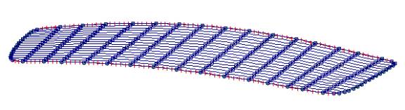
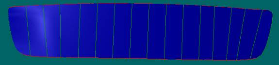
21. Since the surface is drawn in a washed out blue-gray color, I want to change it to a different color. You do this by putting the cursor along any row or column of the surface (not near any edit points) and picking the right mouse button. A dialog box will appear that allows you to change the color. After making the color change, I drew the surface in the 3D view and this is what I got.

The surface might look good, but you really need to examine how the surface matches up to the original digitized points.

22. Display the surface in the Top View again and use the Zoom command to focus on one of the corners of the surface, as shown below. This is where the biggest corrections will be.

When the program fits a surface to the curves, it tries to do its best, but there are always some funny little curves unless the original cross-sections were very nice.

23. Select the Edit-Move Point command. That command is also on the toolbar and is draw with an icon that shows 4 arrows pointing in the 4 main directions. If you select this command, you can grab and drag the bad surface point to fix the shape of the corner of the boundary.

This picture shows the shape of the corner after the surface point was moved a little bit.

You can zoom or scroll all along the boundary edge and fix up all of these little problems. If you don’t think that the surface fit was close enough to the original data, you might want to delete the surface, add more cross-section lines and then re-skin/loft the surface using more curves.

Before you do this, however, I need to talk about accuracy. When you digitized the original shape, you have to have some idea of what kind of accuracy you want. Digitized points always wiggle one way or the other unless you have some nice line or curve that you are following. Even so, you still might have some wiggles in the original data. The skinning/lofting process eliminates some of the wiggles in the raw data (as you can see if you zoom in along the boundary edge), but is it good enough? This is something you will have to decide.

If you want additional accuracy, you might want to smooth or fair the original digitized data first, before you get into the skinning process. Since the original data was in the form of a polyline, there is no easy way to smooth this data. However, Pilot3D includes the ability to fit (interpolate) a smooth curve through the data points. This is done using the Curve-CurveFit command. So, at the very beginning of this process, you could have used this command on the original, single polyline digitized points to create a smooth curve. The smooth curve would have wiggles, but Pilot3D gives you commands for smoothing and fairing curves. If you don’t like the accuracy of the original digitized points, you might want to do this. If so, then you can refer to one of our tutorials on shaping and fairing (smoothing) curves and surfaces.

Since the Skin/Loft command does its own smoothing and since you can go along the edge of the surface and easily fix up problem areas, there is probably no need to smooth or fair the original data.

24. Select the View-Render View-Open Render View command and use the rotation buttons on the toolbar to see what the surface looks like, as shown below. To exit the Render View, pick the ‘X’ in the corner of the window.

After you have fixed up the edges of the surface and checked for accuracy of shape, you are ready to unwrap or develop the shape of the plate.

25. Select the Develop-Develop Plate command and pick one of the rows or column lines of the surface in Top View. A dialog box will appear showing a list of options. This tutorial is long enough, so I won’t go into an explanation of all of the options (see the manual for details).

The most important options are the number of grid rows and columns. Pilot3D uses a finite analysis method for the solutions and this grid is used to subdivide the surface at locations where the strain is calculated. If these values are too high, then the calculation will take a long time. Pilot3D generates a HUGE matrix that is solved based on the grid size. If the program looks like it is taking a long time to do the calculation (see the status line for progress information), then you can press the ESC key to terminate the calculation. Then, you can pick the surface again and enter smaller numbers for the number of grid rows and columns.

For this example, I put in 20 for the number of grid rows and 100 for the number of grid columns. I left the rest of the options alone and picked the OK button. Depending on your machine and how many rows and columns you define, this calculation could take a while. For my not too fast machine, it took about 30 seconds. Check the status line for progress in the solution. The program uses an iterative method of solution and it shows you which step of the solution it is in. If it seems to be taking too long, press the ESC key and pick the surface again. Then, you can try a different combination of grid rows and columns.

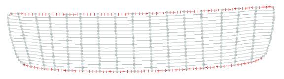
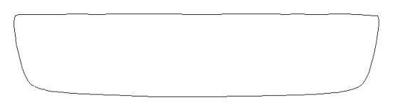
The result of this layout process is calculated and displayed, as shown below.

26. Select the File-Data File Output-DXF Output next if you want to output this boundary shape to a DXF file to send to the CNC cutter software. When the program displays the DXF output dialog box, make sure you select the 2D output option so the program will output what appears on the screen rather than a 3D mesh of the surface.

Conclusion

The key to this process is to fit a surface to the boundary shape because surfaces can be unwrapped, but not wireframe curves. To create a 3D surface with existing data, you need to construct a series of cross-section curves that define the shape of the surface. Once you fit these sections with a surface using the Skin/Loft command, you need to “fix-up” the surface before doing the final unwrap and export to a DXF file.