Reverse Engineering
Example 1
This is an example describing the steps taken to read in raw data
from a DXF file, to fit a NURB surface to the data, and to unwrap the surface
into its 2D pattern for CNC cutting.
The unique aspect of the data is that it includes a radiused corner
cutout on the pattern. These steps
come from a real example and the data comes from a Romer 3D digitizing arm ( www.romer.com ) that was used to digitize a
damaged section of a ship.
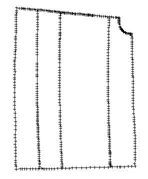
1. Read in the DXF file using the File-Data File Input-DXF Input
command, using all of the default input choices, including the generation of a
TXT input report file. This is what is
shown in the top view of the input data.
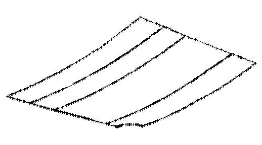
This is what is shown in the 3D view. The data can be rotated to any angle to better understand the
defining shape.
After the DXF file is read, the program displays a summary box
that says that the input data consists of 8 polylines. The following is the last part of the TXT
input report file that gets generated.
…
…
…
Entity
Position 8 - 3D POLYLINE
RGB=(0,0,0)
layer=1
Dimensions=3
Npts = 39
Entity
Position 9 - 3D POLYLINE
RGB=(0,0,0)
layer=1
Dimensions=3
Npts = 58
TOTALS
Entities
Found in C:\RevEngr1.dxf
POINT
Entity - 0
LINE
Entity - 0
POLYLINE
Entity - 8
SPLINE
Entity - 0
MESH
Entity - 0
************* End of Report *************
2. After reading any input data file (DXF, IGES, etc.), the first
thing you need to do is to identify all of the entities and where they are
located. Just because a group of points
looks connected as a single entity, it doesn’t mean that they are. The best way to locate the entities is to
change their colors. Our goal here is
to skin or fit a NURB surface to the 5 cross-section polylines, so let’s change
their colors to blue. This can be done
by clicking the right mouse button on each of the cross-section polylines. A dialog box will appear that allows you to
change the color of the polyline. You
may have to zoom in on the polylines because if you right click too near a
point, the program will display an edit box for the point, rather than the
attribute box for the polyline. You can
also use the Curve-Curve Attribute command.
In this file, each of the cross-sections is one, complete polyline. If, however, only part of the cross-section
changed its color to blue, then you would know that the cross-section is made
up of two or more polyline pieces. If
this was the case, you would have to zoom in on the joining point of the two
pieces and use the Curve-Join Curve command to join the two separate polyline
cross-section pieces into a single polyline entity. We need to make sure that each of the cross-sections is one
complete polyline so that the NURB surface skinning command will work
correctly.
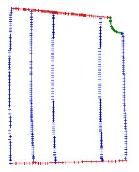
After the cross-sections are changed to blue, we changed the edge
polylines to red and the cutout radius to green. The results are shown below.
Notice that there are 8 polylines that define the input data: 5
cross-section blue polylines, 2 red edge polylines, and one green radius
cutout.
3. Before we can skin the blue cross-sections, we need to fix one
thing. NURB surfaces like to be created
as rectangular-like shapes and they cannot deal with cutouts all by
themselves. Therefore, we need to
pretend that the cutout is not there and extend the edge polylines to the
imaginary rectangular corner point. The
cutout will be dealt with later as a cutout of the NURB surface.
4. Display the polylines in the top or "plan" view.
5. Zoom in on the radius corner of the plate.
6. Select the Move Point command and move (extend) the last point
on the top red line to the right. You
want to move it to the imaginary hard corner of the plate, as if the cutout
wasn't there. [You can use the Hide
Entity command to turn off the cutout radius polyline while you do this step.]
You want to leave the cutout radius curve alone and create the missing corner
of the plate. We have to create a full
rectangular-like surface to get the surface skinning/lofting command to work
well. You will deal with the cutout
after the full surface has been lofted.
7. Do the same with the right side top blue point and extend it to
the imaginary hard corner of the surface.
You can use the Edit-Merge PntToPnt command to merge the two end
polyline points that you have moved to the imaginary corner. That way, you will be able to move both of
them at the same time.
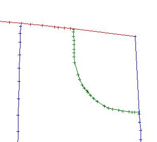
8. Display and zoom in on this corner and adjust its position in
all three views: Profile, Plan, and Section views. Your results should look like this:
9. Next, display the full view of the plate in the top or plan
view. Zoom in on the ends of each of
the blue sections and extend the end points to meet the red side lines. Repeat this process in the profile and
section views. (You can just use the
Edit-Fix Pnt to Curve command to fix the ends of the blue section curves to the
red side curves.) Remember, you don't
have to be perfectly exact. Keep in
mind the accuracy you are dealing with so that you do not "fuss" with
the data too much.
10. Use the Skin/Loft command to fit a surface to the blue section
curves. I told the program to use 20
rows to create the surface. This means
that the program will spread 20 defining rows (equally spaced) along each of
the blue section polylines. You could
use more rows for a more accurate fit to the input data, or you could use fewer
rows for a smoother fit of uneven input data.
The result of the skinning with 20 rows is shown below. Notice that the
program interpolates the sections and creates a true NURB surface with edit
points that lie on the surface. Each
edit point that lies on the surface corresponds to one defining vertex point of
the NURB surface. You can edit the
shape of the surface directly by moving these points.
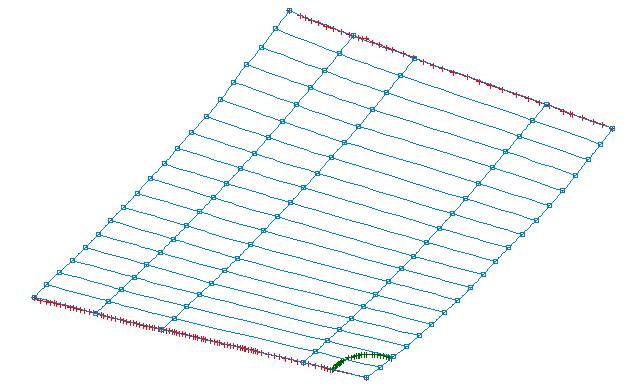
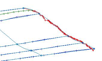
This picture shows how well the interpolated surface fits the
original data. The original input data
is not fair because it came from a damaged section of a ship. It is up to the user to decide if there is a
need to fix up this input data. Later
on, we talk about the choice of fairing or smoothing the curves before the
Skin/Loft command or fairing the surface after the Skin/Loft command. Note that after skinning, the original blue
section curves are turned off. You can
turn them back on (Curve-Draw All Curves) to see how well the surface fits the
raw input data. If the fit is poor, you
can use the Undo command and reskin with more rows. Keep in mind the accuracy you are dealing with.
11. Now, display the plate in plan or top view and zoom in on the
cutout corner.
12. Use the Curve-Curvefit command to fit a curve to the green
cutout polyline.
13. Use the Curve-ReFit Curve-Equal Spacing command to refit the
green curve with fewer points. This
will smooth out the curve and make the next step easier. I used 10 points for this step.
14. Now, you want to "attach" the curve to the
surface. The curve already looks like
it is on the surface, but we have to tell the program to attach it to the
surface. Use the Edit-Fix PntToSurf
command and attach each green curve point to the surface. For each point, this command wants you to: FIRST pick the point that you want to attach
to the surface, and SECOND pick the position on the surface where you want to
attach the point. In this top or plan
view, this means that for each point, you want to carefully position the cursor
on top of the curve point and click the left mouse button twice - first to
select the curve point and second, to attach it to the surface AT THAT SAME
POSITION. Remember to look at the
status line to see whether the program is expecting you to pick the curve point
or to pick a point on the surface. Be
careful not to get out of sync when you are attaching each point on the
surface. Remember, if something doesn't
work correctly, use the Undo command and start over. Continue this process until all green curve points are attached
to the surface. (You could project the
curve to create a surface, then turn on the surface intersection, then attach
the SSI to the surface, then use that for the trim curve, but fixing each point
to the surface, one at a time is simpler and faster.)
15. Zoom in on the ends of the green curve and extend the ends to
the sides of the surface. You don't
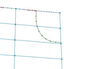
have to be exact here, since the program can deal with small gaps.) Note that since the curve is now attached to
the surface, the program will not let you move the point off of the
surface. This is what the curve on the
surface should look like after attachment.
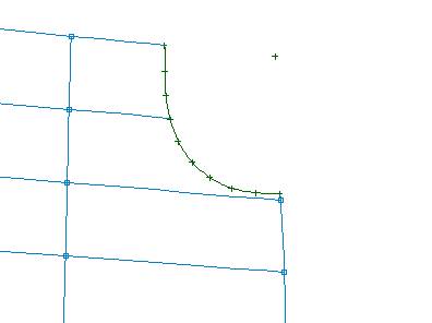
16. Use the Trim Surface command to pick the curve first and then
pick the surface in the corner you wish to cut off. The surface should look like this:
This is the full view:
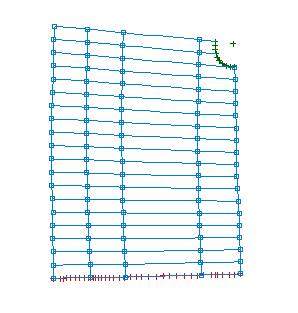
Notice the point at the trimmed off corner of the surface. The program uses this point to create a
closed loop polygon for the NURB surface trim curve. If desired, you can drag or move this or any other green polyline
point to dynamically create a new trimmed shape. The program allows dynamic editing of trimming curves. In this example, this is not necessary.
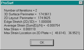
17. Now, select the develop plate command to unwrap the surface to
its 2D shape using all of the develop plate dialog box default options. This is the report that gets generated after
flattening out the plate. The program
uses a finite element type of analysis to determine the strains on the plate
during the flattening process. This
means that the program can flatten both developable surfaces and plates with
double curvature. The default option is
to make sure that the perimeter girth distance of the 2D pattern is the same as
the perimeter girth distance of the 3D surface. This can be adjusted to try to reduce the average strain
(stretch) on the plate.
This is the final, flattened shape of the plate, including the
cutout.
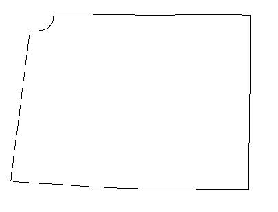
18. While this 2D pattern shape is shown on the screen, select the
File-Data File Output-DXF Output command. When the output options dialog box is
displayed, change the output to "2D View Output", which will output
the current 2D view on the screen to a DXF file.
This whole process took less than 1/2 hour to complete.
Note 1. I did not talk
about massaging or fairing the input data, since I did not know enough about the
accuracy of the input data or how to correct it. Also, even if the input data is accurate, it may not represent
the shape that you want to unwrap. If
the input data is affected by damage or other influences, you may want to use
your judgment in modifying the shape of the input data. Fairing or smoothing can be done in one or
two places. First, you can use the
CurveFit and ReFit Curve commands to reduce and smooth the input
polylines. Then you can use the K-curve
fairing tools to provide further curvature fairing. All of this can be done before you fit the surface to the blue
section curves. The other place that
you can do fairing or smoothing is after the surface has been lofted. You can view the Gaussian curvature of the
surface or display the K-curves of the surface rows and cols and use the
program's fine-tune Move% command to perform detailed fairing. Keep in mind, however, what accuracy you are
trying to achieve.
Note 2. When you digitize objects, you may want to
over-digitize the object to create a nice "rectangular" pattern of
section shapes that you can skin or loft.
(This makes the skin/loft command work very nicely.) Then you can digitize the details separately
to use for the trim surface cutout shapes.